Rational Formulas and Variation

Learning Objectives

• Solve a formula for a specified letter.
• Identify direct, inverse, and joint variation.
• Find the unknown in a variation problem.
• Solve application problems involving direct variation.
• Solve application problems involving inverse variation.
• Solve application problems involving joint variation.

Rational formulasA formula expressed as a rational equation. can be useful tools for representing real-life situations and for finding answers to real problems. Equations representing direct, inverse, and joint variation are examples of rational formulas that can model many real-life situations. As you will see, if you can find a formula, you can usually make sense of a situation.

When solving problems using rational formulas, it is often helpful to first solve the formula for the specified variable. For example, work problems ask you to calculate how long it will take different people working at different speeds to finish a task. The algebraic models of such situations often involve rational equations derived from the work formula, `W = rt`. The amount of work done (`W`) is the product of the rate of work (`r`) and the time spent working (`t`). Using algebra, you can write the work formula `3` ways:

`W = rt`

Find the time (`t`). `t=W/r` (divide both sides by `r`)

Find the rate (`r`). `r=W/t` (divide both sides by `t`)

Now let’s look at an example using the formula for the volume of a cylinder.

Variation equations are examples of rational formulas and are used to describe the relationship between variables. For example, imagine a parking lot filled with cars. The total number of tires in the parking lot is dependent on the total number of cars. Algebraically, you can represent this relationship with an equation.

The number `4` tells you the rate at which cars and tires are related. You call the rate the constant of variationRepresented by the variable `k` in variation problems, the constant of variation is a number that relates the input and the output. . It’s a constant because this number does not change. Because the number of cars and the number of tires are linked by a constant, changes in the number of cars cause the number of tires to change in a proportional, steady way. This is an example of direct variation A type of variation where the output varies directly with the input. Direct variation is represented by the formula `y=kx`., where the number of tires varies directly with the number of cars.

You can use the car and tire equation as the basis for writing a general algebraic equation that will work for all examples of direct variation. In the example, the number of tires is the output, `4` is the constant, and the number of cars is the input. Let’s enter those generic terms into the equation. You get:

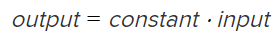
That’s the formula for all direct variation equations.

Let’s find a general way to represent direct variation. When we start talking about input and output in an equation, we often call the equation a function. The output of a function (equation) is also known as the dependent variable and is generally represented symbolically as `y`. The input is called the independent variable, represented by the symbol `x`. Let’s represent the constant with the letter `k`. Now put those symbols into the equation.

`y=kx`

And you’ve done it! All direct variation equations can be described by the equation `y = kx`.

Let’s look at another example of direct variation. Mary works at a roadside stand on the family chicken farm, selling eggs for `$1.99` per carton on busy weekends. When customers buy a lot of cartons at once, she has to add up the totals with a pencil and paper, and she worries about making mistakes. Lucky for Mary, this is a direct variation relationship: the output (total cost) equals the input (number of cartons) times a constant (the price per carton). She can use a direct variation equation to make a pricing table to use as a shortcut.

In this case:

Let’s graph the egg cost/carton function.

This function is made up of individual points because the farm stand only sells whole cartons of eggs. But you can see that all of the points are evenly spaced, and appear to lie on a straight line. You can also see that although it isn’t plotted, the point `(0,0)` satisfies the function. The cost of `0` cartons would be `0` dollars.

Now let’s look at the graph of a continuous direct variation equation and see how it differs from the graph above. (In the graph of a continuous function, individual data points exist at every point along the line, unlike in the egg example above where it makes no sense to talk about the price of `1.235` cartons of eggs!)

Imagine a faucet pours water into a tub at a rate of `2.5` gallons per minute. The amount of water in the tub varies directly with the amount of time the faucet has been running. You can represent the relationship between the time and the water in the tub with the following formula.

Using `g` to represent total gallons of water and `t` to represent time, you may abbreviate this relationship as `g = 2.5t`, which looks very similar to the standard formula for proportional functions, `y = kx`.

Let’s make a table to chart the relationship of time versus the amount of water in the tub. After `1` minute, `2.5` gallons are in the tub. After `2` minutes, the total is `5` gallons, and so on. To find the total amount of water in the tub at any time, you can multiply the time by `2.5` gallons per minute. Six minutes should give you enough points to make a useful graph.

Now you can graph those points.

This time, use a line to connect the points, because both time and water increase continuously. The points lie on a straight line that begins at the origin and rises at a steady angle, just like the last graph. In the egg example, it didn’t make sense to purchase `2.5` cartons of eggs, so you did not draw a line to connect the points. But with the water example, you can measure the total number of gallons after `2.5` minutes, so connecting the points makes sense.

When the variables in a function change at a constant rate like this, they have a proportional relationship. This steady rate of change is called the constant of variation.

Another kind of variation is called inverse variationA type of variation where the output varies inversely with the input. Inverse variation is represented by the formula `y=k/x`. . In these equations, the dependent variable equals a constant divided by the independent variable. In symbolic form, this is the equation `y=k/x`, where `y` is the dependent variable, `k` is the constant, and `x` is the independent variable. Compare this with the equation for a function that has direct variation between the variables, such as the direct variation formula of `y=kx`. The only difference is that the independent variable is now in the denominator.

One example of an inverse variation is the speed required to travel between two cities in a given amount of time.

Let’s say you need to drive from Boston to Chicago, which is about `1,000` miles. The more time you have, the slower you can go. If you want to get there in `20` hours, you need to go `50` miles per hour (assuming you don’t stop driving!), because `(1,000)/20=50`. But if you can take `40` hours to get there, you only have to average `25` miles per hour, since `(1,000)/40=25`.

The equation for figuring out how fast to travel from the amount of time you have is `"speed"=("miles")/("time")`. This equation should remind you of the distance formula `d=rt`. If you solve `d=rt` for `r`, you get `r=d/t`, or `"speed"=("miles")/("time")`.

In the case of the Boston to Chicago trip, you can write `s=(1,000)/t`. Notice that this is the same form as the inverse variation function formula, `y=k/x`.

Here’s a table that shows several times and speeds that satisfy the equation:

Now if you plot those points, you’ll see that the graph is definitely a curve, not a line.

A third type of variation is called joint variationA type of variation where the output varies jointly with multiple inputs. Joint variation is represented by the formula `y=kxz`. Joint variation is the same as direct variation except there are two or more quantities. For example, the area of a rectangle can be found using the formula `A = lw`, where `l` is the length of the rectangle and `w` is the width of the rectangle. If you change the width of the rectangle, then the area changes. Similarly, if you change the length of the rectangle, then the area will also change. You can say that the area of the rectangle “varies jointly with the length and the width of the rectangle.”

The formula for the volume of a cylinder, `V=pir^2h` is another example of joint variation. The volume of the cylinder varies jointly with the square of the radius and the height of the cylinder. The constant of variation is `pi`.

Finding `k` to be `1/2` shouldn’t be surprising. You know that the area of a triangle is one-half base times height, `A=1/2bh`. The `1/2` in this formula is exactly the same `1/2` that you calculated in this example!

It is important to be able to distinguish if an application is varying directly, inversely, or jointly.

Rational formulas can be used to solve a variety of problems that involve rates, times, and work. Direct, inverse, and joint variation equations are examples of rational formulas. In direct variation, the variables have a direct relationship: as one quantity increases, the other quantity will also increase. As one quantity decreases, the other quantity decreases. In inverse variation, the variables have an inverse relationship: as one variable increases, the other variable decreases, and vice versa. Joint variation is the same as direct variation except there are two or more variables.