
Graphing Systems of Inequalities
In a system of equations, the possible solutions must be true for all of the equations. Values that are true for one equation but not all of them do not solve the system. The same principle holds for a system of inequalitiesA set of two or more inequalities that must hold true at the same time., which is a set of two or more related inequalities. All possible solutions must be true for all of the inequalities.
Because even a single inequality defines a whole range of values, finding all the solutions that satisfy multiple inequalities can seem like a very difficult task. Luckily, graphs can provide a shortcut.
The graph of a single linear inequality splits the coordinate plane into two regions. On one side lie all the possible solutions to the inequality. On the other side, there are no solutions. Consider the graph of the inequality `y<2x + 5`.
The dashed line is `y = 2x + 5`. Every ordered pair in the colored area to the right of the line is a solution to `y<2x + 5`. Skeptical? Try substituting the `x` and `y` coordinates of Points A and B into the inequality—you’ll see that they work.
The colored area, the area on the plane that contains all possible solutions to an inequality, is called the bounded regionThe set of solutions that are true for all of the linear inequalities under consideration.. The line that marks the edge of the bounded area is very logically called the boundary lineA line that represents the edge of a linear inequality: if points along the boundary line are included in the solution set, then a solid line is used; if points along the boundary line are not included in the solution set, then a dashed line is used.. In this case, it was dashed because points on the line don’t satisfy the inequality. If they did, as they would have if the inequality had been `y<=2x + 5`, then the boundary line would have been solid.
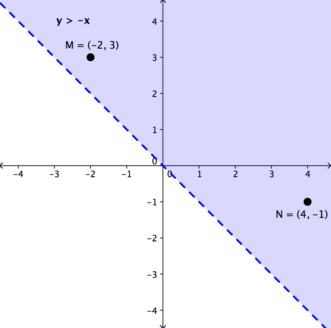
Let’s clear the grid and graph another inequality: `y> -x`. This inequality also defines a half-planeOn a coordinate plane, the shape of the region of possible solutions generated by a single inequality.. The points `M` and `N` are plotted within the bounded region. This means that both points yield true statements when their `x` and `y` coordinates are substituted into the inequality `y> -x`.
To create a system of inequalities, we need to graph two or more inequalities together. Let’s use `y<2x + 5` and `y> -x` since we have already graphed them independently.

See the purple area, where the bounded regions of the two inequalities overlap? This is the solution to the system of inequalities. Any point within this purple region will be true for both `y> -x` and `y<2x + 5`. Both inequalities define larger individual bounded regions, but the range of possible solutions for the system will consist of the smaller bounded region that they have in common.
On the graph, you can see that the points B and N provide possible solutions for the system because their coordinates will make both inequalities true statements.
In contrast, points M and A both lie outside the shared bounded region. While point M is still a possible solution for the inequality `y> -x` and point A is still a possible solution for the inequality `y<2x + 5`, neither point is a valid solution for the system.
In order to figure out whether a given point is a solution for a system of inequalities, we can look to see whether it lies within the common region for that system. Let’s look at a few examples.
Determine whether `(3, -2)` is a possible solution for the system:
`y>0.5x-2`
`x + y<=5`
Before even graphing this system, we can substitute the values `x = 3` and `y = -2` into each inequality and see if we get true statements. This is a quick way of determining whether the given point is a solution for the system (although we will graph this system as well).
|
`y>0.5x-2` |
`-2>0.5(3)-2` |
`-2>1.5-2` |
`-2> -0.5` |
false statement |
|
`x + y<=5` |
`3 + (-2)<=5` |
`3-2<=2` |
`1<=2` |
true statement |
We get one true statement and one false statement, which means that this point will not be a solution for the system, although it will work for one inequality.
Now let’s graph the system to see where this point lies, and where the bounded region is. To graph the system, we will graph each inequality. First we graph the boundary line for `y>0.5x-2` and shade the region above the line (shown in pink in the image below) since points in that region make the inequality true.
Next we graph the boundary line for `x + y<=5`, making sure to draw a solid line because the inequality is `<=`, and shade the region below the line (shown in blue) since those points are solutions for the inequality. The region on the upper left of the graph turns purple, because it is the overlap of the solutions for each inequality. This is our solution set for this system.

The point in question, `(3, -2)`, lies within the bounded region for `x + y<=5` but outside the bounded region for `y>0.5x-2`. Thus, it is not a solution for the entire system.
|
Which of the points listed below are solutions for the system? `y>x` `x-2<0` `1`. `(1, 1)`
`2`. `(-5, 9)`
`3`. `(0, 7)`
A) `1` and `2`
B) `2` and `3`
C) `1` and `3`
D) `2` only
|
Sometimes a system of inequalities has no solutions. This can happen when the boundary lines are parallel.
Consider the following system:
`y>=2.5x + 4`
`y<2.5x`
A graph of this system is shown below.

The bounded regions of the two inequalities do not overlap, so there is no solution set.
However, the existence of parallel lines does not necessarily indicate that there is no solution, it just means that there is the possibility of no solutions. Using the graph above, think about the graph of the system `y>2.5x` and `y<=2.5x + 4`. A thin band of possible solutions exists between the two parallel lines.
Systems of inequalities can be graphed on a coordinate plane. The solution set for a system of inequalities is not a single point, but rather an entire region defined by the overlapping areas of each individual inequality in the system. Every point within this region will be a possible solution to both inequalities and thus for the whole system. When two inequalities within a system share no common region, then the system has no solution, and no individual point will be a solution set to both inequalities.